When Similarity Isn't Signal
Testing the hidden assumptions behind convincing matches
- Published
- November 16, 2026
- Updated
- November 18, 2026
- Version
- 1.1
Cite this article
Citation
Plain text
Carson, D. (2026). When Similarity Isn't Signal: Testing the hidden assumptions behind convincing matches. Technical report, version 1.1. Vaela. https://vaela.ai/research/when-similarity-isnt-signal
BibTeX
@techreport{carson2026when,
  author = {Carson, Davis},
  title = {{When Similarity Isn't Signal: Testing the hidden assumptions behind convincing matches}},
  institution = {Vaela},
  year = {2026},
  month = {nov},
  note = {Version 1.1. Not peer reviewed},
  url = {https://vaela.ai/research/when-similarity-isnt-signal}
}AbstractA retrieval system can return an answer for every query and still fail to predict the quantity we care about. We investigated an archived visual-personalization prototype and found that returning a close match, finding a predictive signal, and making a useful recommendation are three different achievements. Only the first is guaranteed by the software.
- Evaluation
- Retrieval
- Personalization
A retrieval system can return an answer for every query and still fail to predict the quantity we care about. We investigated an archived visual-personalization prototype and found that returning a close match, finding a predictive signal, and making a useful recommendation are three different achievements. Only the first is guaranteed by the software.
Evidence and scope. Every number in Sections 3 to 7 was recomputed on 2026-11-11 from retained data files, using a new script written for this study. The first version of the prototype's retrieval code was not preserved, so one early single-query diagnostic could not be reproduced and is not used here. Outside publications give methodological context. They do not verify our findings. We distinguish measured results from conceptual illustrations and from proposed follow-up experiments. Application-specific measurement identities and extraction details are withheld, so this article is not sufficient for independent reproduction.
#1. A match is easy to find. A reason to trust it is harder.
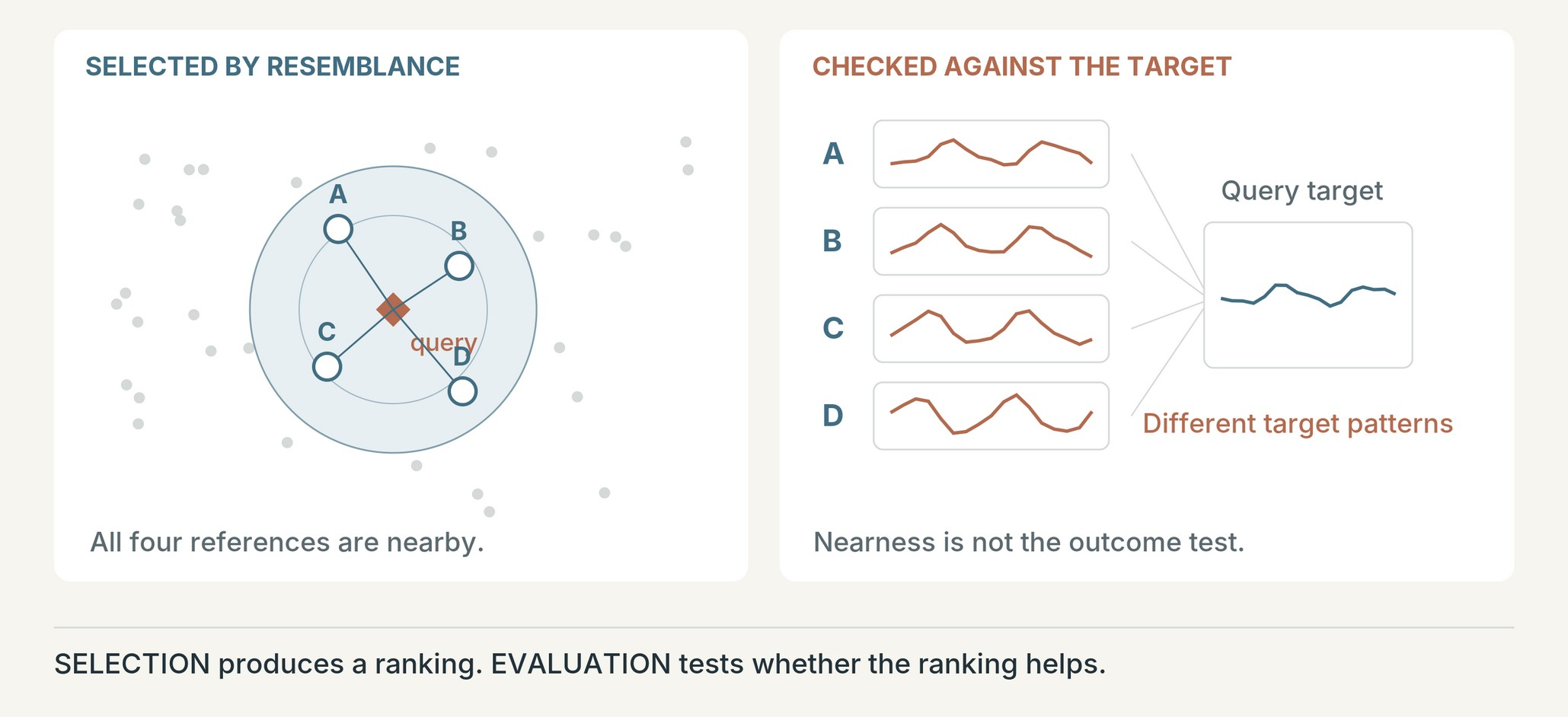
Suppose a system is asked for examples that resemble a new observation. It returns a ranked list. The first example is closer than the second, the second closer than the third, and every item has a score. Nothing is visibly broken.
It is tempting to read that order as evidence that the system has understood something. But the ranking answers a narrower question: which available examples are closest under this representation and this distance rule? It does not answer whether those examples tell us anything about another quantity.
For any nonempty reference set and any defined distance, some example is closest. That stays true when the representation is poorly chosen, when query and reference measurements are incompatible, and when the dominant variation has nothing to do with the intended prediction. The system does not need a meaningful relationship to produce a convincing list.
This mattered in an archived visual-personalization prototype. The prototype used image-derived measurements to select reference examples, then used those examples to estimate a separate visual target. The hypothesis was simple: selecting references by resemblance should improve the estimate compared with selecting references at random.
We did not treat a plausible output as evidence for that hypothesis. We compared the two selection strategies on the same query images, ran randomized controls, and tested whether a shared imaging influence could explain part of the apparent relationship. The result was more complicated than a broken model becoming a working one.
In the original index, the nearest-reference estimate was not distinguishable from its shuffled-target control. In a later, consistently measured index, the association was much larger, but about 60 percent of its advantage over random selection (22.5 points of win rate above the 50 percent reference, reduced to 9.1 points) disappeared when we adjusted for a proxy of shared acquisition conditions. A smaller association remained. None of this shows that people would prefer the system's recommendations.
This article is about the gap between a system producing an answer and an experiment establishing what the answer means. The application is one concrete case. The questions apply whenever resemblance in one space is used to justify a prediction in another. We do not claim a new general theory of retrieval. We report how familiar evaluation problems can coexist inside a functioning pipeline.
The diagnostic question is also current in published work. A 2026 study of multimodal recommendation keeps model architectures intact and replaces selected embeddings with constants or noise, to test whether the claimed input information contributes to performance [1]. Its results vary by architecture and do not show that visual representations are generally unhelpful. A 2026 editorial on recommender evaluation likewise stresses well-tuned baselines and inspectable experimental procedures [5]. That is guidance on how to establish evidence, not support for the measurements reported here.
#2. Three hidden assumptions inside a similarity score
The prototype relied on assumptions that a distance calculation cannot check.
The query and the references must be measured in the same way. Two descriptors can have the same shape and different meanings. One may be a raw measurement and the other a normalized or transformed version of it. The software accepts both and computes a valid distance. The comparison is still wrong, because the numbers are not on the same scale or in the same units.
The representation must keep the information the target needs. A transformation can help one task and hurt another. Removing one source of variation makes some predictions easier and can remove a distinction a different prediction needs. A narrow numerical range does not by itself prove information loss, because an invertible rescaling can compress values and keep their order. What matters is the relationship among the transformation, the estimator, and the target.
The association must mean what we think it means. Two measurements taken from the same image can move together because of shared acquisition conditions. A system can use that association, score well on an internal prediction task, and never recover the relationship the product was built around.
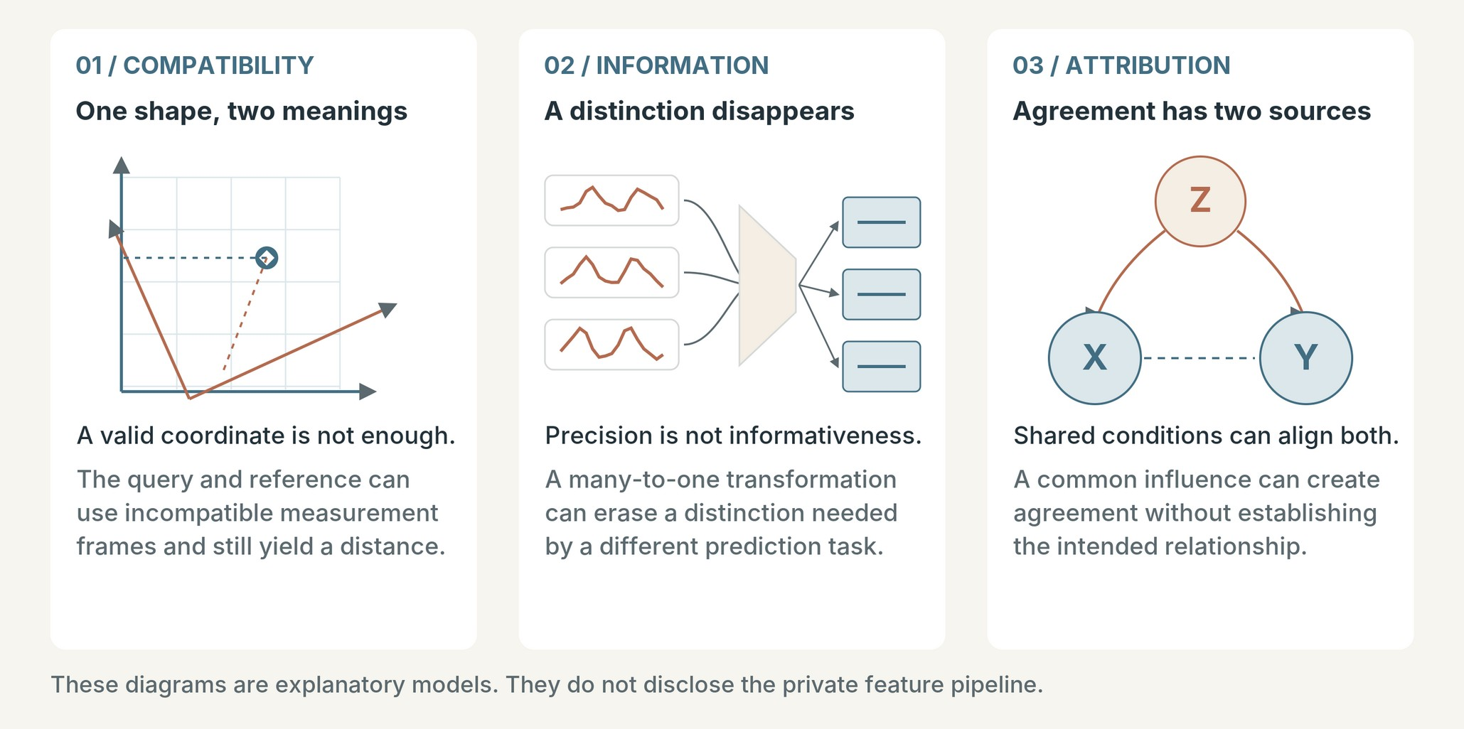
These assumptions interact. A representation mismatch can hide a weak real relationship. Repairing the mismatch can expose a stronger correlation that is partly driven by a nuisance factor. Finding one problem does not rule out another, and a better score does not say which assumption has become more defensible.
For that reason a before and after comparison is not enough. Each control has to answer a distinct question. Recent work on auditing representations makes a related point: a 2026 study analyzes embedding geometry and the changes fine-tuning induces, to expose spurious features that prediction-based checks can miss [2]. Its methods and settings differ from ours. It is context for inspecting a representation instead of assuming that plausible outputs show what a system relies on.
#3. An experiment that asks whether selection matters
The evaluation used 479 synthetically generated images. Each image has an input descriptor and a separate target measurement. Each image was used in turn as the query and excluded from its own reference pool. For each query we estimated the target as the mean target of the twelve nearest references. The comparison estimate was the mean target of twelve references drawn at random. We drew 100 random sets per query.
The same query and the same target appear on both sides of the comparison. Changing the query set or the target at the same time as the selection rule would make the result harder to interpret. The comparison is informed selection against random selection, with everything else held fixed within one evaluation.
For query i, let yi be its target and L the error rule of that evaluation. For random draw b, define
where ŷNi is the estimate from the nearest references and ŷRib is the estimate from random references. A positive Δ means the nearest references gave the smaller error. The win rate is the fraction of (i, b) pairs with Δ > 0, averaged over draws and then over queries. Ties count as losses. This notation describes the computation. It is not a copy of the code.
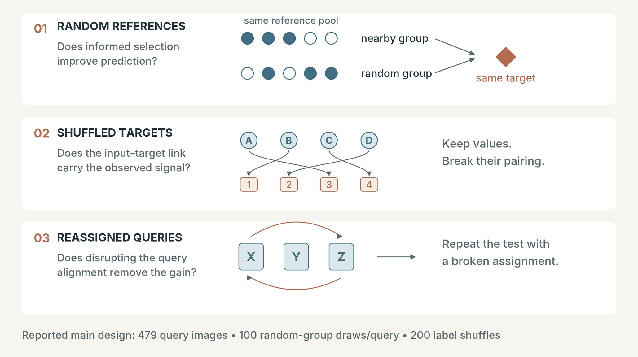
The random-group comparison and the shuffled-target comparison answer different questions. Random groups give an alternative prediction for each query. Shuffling targets across images shows what the statistic looks like when the link between descriptor and target is broken and the set of target values stays the same. We used 200 target permutations for the main null comparisons, with the neighbor sets held fixed. We report permutation p-values as (1 + number of shuffled statistics at least as large as the observed one) divided by (1 + 200), following the standard recommendation that a randomly drawn permutation p-value cannot be zero [6]. The smallest possible value is therefore 1/201, about 0.005.
We report 95 percent bootstrap intervals that resample query images 2000 times. In this image set each image is its own cluster, so this is a cluster bootstrap with one image per cluster [7]. The intervals and the shuffled-target ranges describe different things. An interval describes uncertainty in the observed statistic under resampling. A shuffled-target range shows where the statistic falls when the input and target are unlinked. A chart that draws both without saying so is confusing.
A value of 50 percent is a useful visual reference, but it is not a substitute for the empirical null. The two strategies need not have identical distributions in a finite dataset, and the same reference pool is reused for every query. The shuffled results are part of the evidence.
#4. The baseline changes the story
The original index won 52.5 percent of comparisons. The 95 percent bootstrap interval was 49.8 to 55.4 percent. The middle 95 percent of its shuffled-target statistics ran from 44.8 to 53.7 percent, and the permutation p-value was 0.14.
This does not show the true effect is zero. It shows that this evaluation did not separate the observed result from the randomized comparison, and a small effect fits within the interval. The supported conclusion is narrow: we did not establish a reliable predictive advantage for this condition under this test. It is not "similarity does not work."
The retrieval itself still functioned. It returned references and fed a downstream output. The failure was not a crash, an empty result, or a nonsensical answer. We could not show that the selection rule contributed information about the target.
A second index, with the query and the references measured the same way, gave a larger result after our nuisance adjustment: 59.1 percent, with a 95 percent interval of 56.0 to 62.1 percent. Its shuffled-target range was 47.4 to 52.4 percent, and its permutation p-value was 0.005, the smallest value 200 shuffles can give.
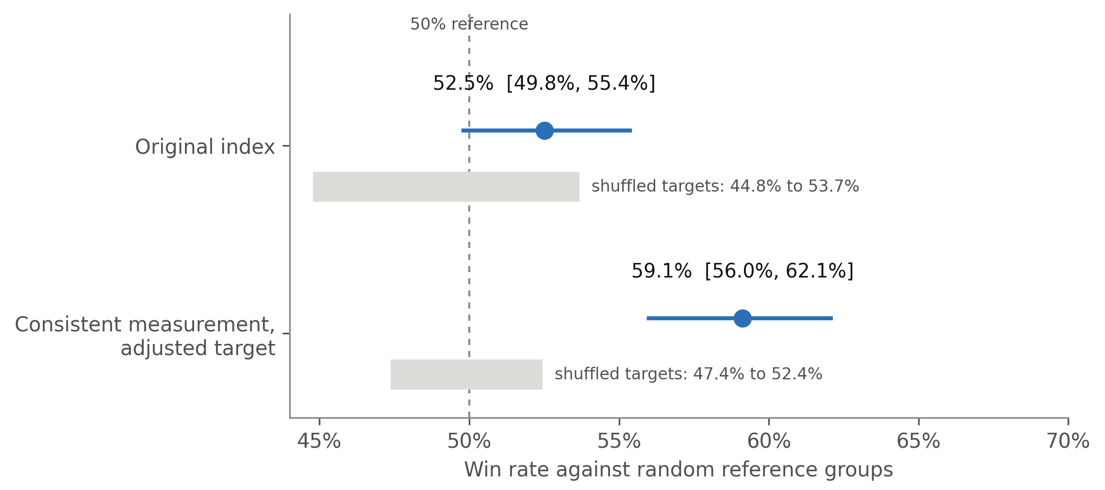
The two estimates can only be placed side by side with their limits in view. They do not isolate one intervention. The measurement of the query and the references changed, the target changed, and the error rule changed: the original-index evaluation used a different distance between estimate and target than the other two. Calling the gap between 52.5 and 59.1 percent the effect of "fixing the representation" would claim a controlled comparison the data do not provide.
The value of the baseline is more modest and more general. It separates a retrieval system that runs from a retrieval strategy with a demonstrated predictive association. That is a stricter standard than asking whether the output looks personalized. It is still a standard about a proxy task, not about whether anyone made a better decision.
#5. The strongest-looking result is not the strongest claim
Before the adjustment, the consistently measured index won 72.5 percent of comparisons, with a 95 percent interval of 69.6 to 75.2 percent. After adjustment, the win rate was 59.1 percent. Both rows use the same distance rule, the same twelve references, and the same images. The adjustment changes the target being predicted: it removes the part of the target that a second measurement from the same image predicts, where that second measurement serves as a proxy for shared acquisition conditions.
The difference is 13.4 percentage points. Measured from the 50 percent reference, the apparent advantage fell from 22.5 points to 9.1 points. These are arithmetic on the two point estimates, not a new experiment. We do not give an interval for the difference, because the two marginal intervals do not determine one.
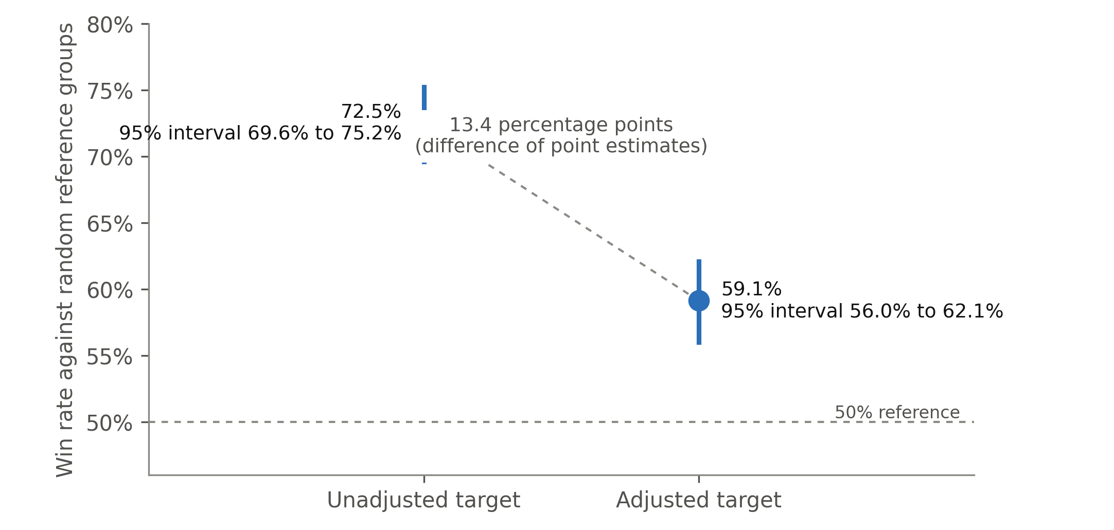
A headline could easily use the larger number: the method beats random selection in nearly three quarters of comparisons. That would leave out the most informative result. The apparent strength of the relationship depends heavily on how shared image-level variation is handled.
We read much of the decrease as consistent with a shared imaging influence. The adjustment may also remove real signal, and we cannot tell the two apart from this data. A proxy adjustment is not an intervention that changes acquisition conditions while holding the underlying observation fixed.
The supported statement is therefore this: a smaller association remained in this synthetic set after one particular adjustment meant to reduce a shared influence. We did not measure how much of the unadjusted advantage was caused by the imaging influence, and we do not know that what remains is the product-relevant signal. A correction can lower a score and make the claim more credible. The word "controlled" still hides the assumptions the control introduces.
#6. What would make the causal explanation stronger?
Two further diagnostics point to plausible explanations of the weak original result. In the original index, the query and the references used descriptors with different measurement meanings, and one stored target dimension had unusually compressed variation. Both could produce misleading retrieval. Neither is a complete causal explanation merely because it appears alongside a weak score.
A low correlation between two versions of a descriptor does not prove one is useless, and a compressed range does not prove information was lost. What matters is whether the transformation preserves the distinctions the task needs and whether the estimator and error rule use those distinctions correctly.
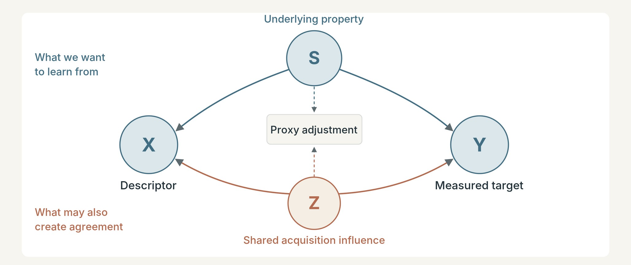
The nuisance problem is subtle. Suppose an unobserved property S contributes to both a descriptor X and a target Y, and an imaging influence Z also affects both. A nearest-reference predictor can benefit from either route. Removing variation associated with a proxy for Z weakens the nuisance route, and it also removes some variation tied to S when the proxy is entangled with it.
A stronger follow-up would vary acquisition conditions for repeated observations of the same underlying subject, with a documented target and appropriate data rights. That would let us ask whether changing the condition changes retrieval while more of the underlying identity is held fixed. A second comparison could hold the target constant and change one representation choice at a time.
These experiments are proposed, not done. They would separate "the metric changed when we adjusted the data" from "we isolated the effect of the nuisance variable." The current record supports the first statement directly and the second only weakly.
#7. What survived nearby tests
A useful result should not depend on one convenient parameter choice. We ran several nearby variations on the consistently measured, adjusted evaluation. All of them used the same 479 images. The first three robustness runs used 100 shuffles and 1000 bootstrap resamples instead of 200 and 2000. The last row uses its own earlier procedure, with its own settings.
| Check | Result | What it supports, and what it does not |
|---|---|---|
| Neighborhood size | Win rates from 57.7% to 60.3% over sizes 1, 3, 5, 12, 25, 50 | The association was not tied to one neighborhood size. This is a range of estimates, not an interval. |
| Alternative ranking distance | Win rate 59.3% | A nearby ranking rule gave a similar value on the same data. This is not an independent replication. |
| Reassigned query descriptors | 50.8%, 95% interval 48.2% to 53.6% | The negative control was consistent with the 50% reference. It does not validate every part of the analysis. |
| Earlier internal test procedure, seven random seeds | Mean 59.5% (range 57.0% to 62.8%), against 49.4% for shuffled targets over 21 runs | A different sampling procedure on the same images agreed. It is not evidence from a new population. |
The pattern is more informative than any one row. The association holds across nearby settings and goes away when the pairing between input and target is deliberately broken. That fits a method using some structure in these data and not one succeeding at a single chosen setting.
There are limits. Every check used the same images, so the results are correlated and are not several independent studies. We cannot say which checks were chosen before seeing the data and which were added after. In the adjusted evaluation, the three terciles of one observed descriptor had overlapping intervals (about 160 images each, win rates 57.3 to 60.2 percent). We do not read that as a fairness result. Small synthetic groups with no detected difference do not show equal performance across real people, capture conditions, or user needs. The generated images are also not an audited sample of any population, and they do not cover all demographic groups.
Robustness should be stated with its domain attached: stable across these settings, in this reference set, under this target and error rule. Removing those qualifiers makes the claim broader without making the evidence stronger.
#8. Reproducibility has more than one layer
The investigation began with a historical single-query diagnostic and later moved to an evaluation over many images. They are separate pieces of evidence. The early diagnostic could not be reproduced exactly, because the first-version implementation was not preserved. When we reconstructed it on the nearest surviving data snapshot, whether real neighbors beat random ones changed with an implementation choice that nobody recorded. We therefore do not use the early diagnostic as a quantitative result. The multi-image results come from retained index files and a script we wrote for this study, and each reported number can be traced to a specific input file and run.
That history should not be flattened into a story where every earlier observation has been rerun. The missing early code also does not invalidate the later measurements. The right response is traceability: each number is tied to the script, input file, and settings that produced it. A 2026 survey of recommender-system reproducibility separates re-running prior work from extending it with new models or evaluation criteria [4]. We keep the same separation. A reconstruction, a rerun, and a new experiment are different activities and we do not call them all "reproduced."
The statistics have layers too. There are 479 query images, and 100 random sets per query do not give 47,900 independent observations. Repeated draws characterize the random comparator for one query. They do not multiply the number of independent images.
The bootstrap resamples query images. That does not account for every dependence. All queries draw on the same reference pool, and generated images may share structure from the generator. Our intervals describe sampling variation over these 479 images given this pool. They do not describe variation over other reference pools or other generators. We screened for near-duplicate images with a perceptual hash and found no pair close enough to be a duplicate. That screen cannot show that every generated image is an independent identity, so the unit of observation here is an image, not a verified distinct person.
Finally, 200 shuffles limit the resolution of the permutation test. A p-value of 0.005 means no shuffled statistic reached the observed one. It should not be reported with extra decimal places. In our shuffles only the target column was permuted. The neighbor sets were fixed and no preprocessing was rerun.
#9. Predictive structure is not yet personal value
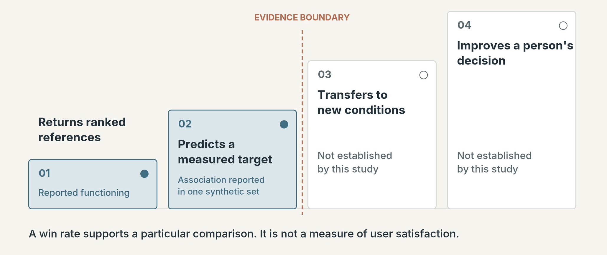
The images are synthetic. Their targets are measurements of generated content, not records of what real people chose, liked, bought, or found useful. The association we tested is structure in a generated dataset. A generator can produce correlations that are stable inside its outputs and mean something different in a natural population.
A 59.1 percent win rate also leaves out the size of each win. A method can beat the comparator by a tiny amount in many trials and have the same win rate as a method whose wins are large. A few large errors can matter in ways a win rate hides. Per-query error differences, calibration, and task-specific costs would be needed to examine that. In the adjusted evaluation, the mean error reduction from using the nearest references was positive, with a 95 percent interval that excluded zero, but we have not studied its distribution or its size in practical terms.
This gives a hierarchy of questions. Does the system return references? Does selection improve prediction of the chosen target? Does the association survive new acquisition conditions or a different dataset? Does it improve the decision a person needs to make? Our study provides evidence for the second question and some within-dataset robustness checks. It does not answer the last two. That is a reason to keep a proxy measurement from becoming a product claim, not a reason to discard the work.
A 2026 study of recommender evaluation compares model rankings from sparse offline data with rankings from denser user-feedback targets. It finds that agreement depends on the dataset and the evaluation design, and that no design is best across its settings [3]. That is not a replication of our study. It shows why an offline comparison needs a justified link to the user outcome being claimed.
This matters most in personalization. The word "personalized" can suggest that a system understands a person's needs when the evaluation showed only that two measured variables are associated. A publication should say where the observation ends and the interpretation begins.
#10. How to make the evaluation portable
The part of this case that transfers is not a private feature recipe. It is a sequence of challenges an apparent matching advantage should survive.
First, establish the value of selection. Keep the query, reference-group size, estimator, and target fixed within a comparison, and replace informed selection with random selection. A random baseline is a cheap way to falsify a claim. It is not an adequate final benchmark for every task. Stronger comparisons include a simple global estimate or other well-tuned predictors, depending on the target [5].
Second, test the measurement contract. Confirm that query and references represent compatible quantities. This is more than a schema check, because two arrays can share a shape and differ in meaning. Versioned measurement definitions, explicit transformations, and controlled comparisons make such differences inspectable without exposing a whole production system.
Third, challenge the association. Break the relationship that is supposed to support the prediction and keep other structure. A shuffled-target test needs an exchangeability assumption to be valid. A nuisance adjustment needs assumptions about what it removes. Calling either a control does not make it trustworthy.
Fourth, test the boundary of the conclusion. Move from nearby settings to new data or real interventions. Then assess user-relevant outcomes separately. These are progressively stronger kinds of evidence and should not be merged into one success label.
A public, task-neutral testbed with known failure mechanisms would make this method easier to inspect. A researcher could build data in which the query and reference coordinates use deliberately incompatible frames, a transform deliberately removes a predictive dimension, or a known common influence affects both input and target. Each manipulation would be labeled and controlled by construction. Such a testbed would be a new experiment, not an anonymized copy of our private results. It would need honest baselines, cases where a control fails, and comparisons that change one mechanism at a time. We have not built it, and no figure here presents simulated results as findings.
#11. What this article discloses and withholds
This article states what was measured, what was compared, and how far the findings reach. It discloses the dataset size and its synthetic origin, the generic prediction comparison, the repeated random-reference draws, the shuffled-target controls, the estimates, the uncertainty summaries, and the main limitations. It withholds the application-specific feature identities, the extraction pipeline, the stored data layout, and the product integration.
That is a real compromise. A reader can check the statistical argument and its limits but cannot rerun the study from this article. We describe this as a bounded applied case study with an internal record of where each number came from. It is not an independently reproduced benchmark and not a validated general theory.
#12. What we can say now
A functioning similarity system produced plausible outputs. In a random-reference evaluation, the original index did not separate clearly from its shuffled-target control. A consistently measured index showed a larger association that fell by more than half, but did not disappear, under one adjustment for shared acquisition conditions. Nearby robustness checks agreed with the smaller remaining association.
The limits are as follows. The data are synthetic. The target is not human preference. The two win rates answer related but different prediction questions. The code for an early diagnostic was not preserved. This article is not enough for independent reproduction.
The general lesson is not that nearest-neighbor methods cannot be trusted. A matching system carries assumptions about what its representations mean, what they keep, and why they agree with an outcome. Those assumptions need experiments of their own.
A ranked list shows that the software runs. A controlled comparison can show that a selection rule carries predictive information. Evidence from a relevant user task is needed to show value. A strong publication keeps these three claims separate, even when one impressive number would be easier to sell.
#References
- Ye, Y., Fu, J., Song, Y., Zheng, K., and Jose, J. M. (2026). A reproducibility study of multimodal embeddings for recommender systems. International Journal of Multimedia Information Retrieval, 15, 14. https://doi.org/10.1007/s13735-026-00408-9. An earlier version appeared as "Are multimodal embeddings truly beneficial for recommendation? A deep dive into whole vs. individual modalities," ECIR 2026, arXiv:2508.07399. ↩
- Păduraru, C. D., Barbalau, A., Filipescu, R., Nicolicioiu, A. L., and Burceanu, E. (2026). Bridging explainability and embeddings: BEE aware of spuriousness. International Conference on Learning Representations (ICLR 2026). arXiv:2410.18970. ↩
- Parajuli, S., Vaez Barenji, S., and Ekstrand, M. D. (2026). On the convergent validity of offline evaluation designs for recommender systems. arXiv:2607.25097. Preprint; the arXiv page does not name a venue. ↩
- Said, A., and Bellogín, A. (2026). Reproducibility in recommender systems: A survey. arXiv:2607.26074. Preprint. ↩
- Jannach, D., and Chen, L. (2026). Improving methodological standards in recommender systems offline evaluation (editorial). ACM Transactions on Recommender Systems, 4(3), Article 34e. https://doi.org/10.1145/3800587 ↩1 ↩2
- Phipson, B., and Smyth, G. K. (2010). Permutation p-values should never be zero: calculating exact p-values when permutations are randomly drawn. Statistical Applications in Genetics and Molecular Biology, 9(1), Article 39. https://doi.org/10.2202/1544-6115.1585 ↩
- Field, C. A., and Welsh, A. H. (2007). Bootstrapping clustered data. Journal of the Royal Statistical Society: Series B, 69(3), 369 to 390. https://doi.org/10.1111/j.1467-9868.2007.00593.x ↩
Version history
- 1.0, November 16, 2026. First release.
- 1.1, November 18, 2026. Figures: removed captions baked into the images. No change to text, data or conclusions.